Unveiling the Magic of Generative Adversarial Networks (GANs)

Welcome to the fascinating world of Generative Adversarial Networks, or GANs for short! Since their introduction by Ian Goodfellow and his team in 2014, GANs have been making waves in the AI community. From creating stunningly realistic images to enhancing photo quality, GANs are doing some pretty magical things. But what exactly are they, and how do they work? Let’s dive in and find out!

What are GANs?

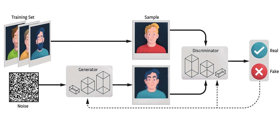
Imagine you have two artists. One is trying to create fake masterpieces, and the other is trying to spot the fakes. This is essentially how GANs work, except our artists are neural networks.
Generator (G): This is our creative artist. It starts with a bunch of random noise and tries to turn it into something that looks real, like an image of a cat or a sunset.
Discriminator (D): This is our critic. It examines images and tries to figure out if they’re real (from a real dataset) or fake (created by the generator).

How GANs Work

The magic happens through a back-and-forth game between these two networks that start with random skills (weights):
Training the Critic: We show the discriminator some real images and some fakes. It tries to correctly identify which is which and gets better at spotting the fakes.
Training the Artist: We give feedback from the discriminator to the generator. The generator tries to create better fakes that can fool the discriminator.
This process goes on, with both the generator and discriminator improving their skills over time. The generator learns to create more realistic images, while the discriminator gets better at spotting the fakes.

The Math Behind the Magic

If you like math, here’s a peek under the hood. The interaction between the generator and discriminator is like a game where each is trying to outsmart the other. This is described by the following equation.
\[ \min_G \max_D V(D, G) = \mathbb{E}_{x \sim p_{\text{data}}(x)}[\log D(x)] + \mathbb{E}_{z \sim p_z(z)}[\log(1 - D(G(z)))] \]
Don’t worry if this looks complex! Let’s break it down:
Discriminator’s Goal: The discriminator tries to maximize its ability to tell real images from fake ones. It does this by maximizing the term \( \mathbb{E}_{x \sim p_{\text{data}}(x)}[\log D(x)] \), which represents the expected value over all real data samples. This term is maximized when \( D(x) \) (the discriminator’s output for real data) is close to 1 (high probability that the data is real).
At the same time, the discriminator also tries to minimize the term \( \mathbb{E}_{z \sim p_z(z)}[\log(1 - D(G(z)))] \), which represents the expected value over all fake data samples. This term is minimized when \( D(G(z)) \) (the discriminator’s output for fake data) is close to 0 (high probability that the data is fake).
Generator’s Goal: The generator, on the other hand, tries to fool the discriminator. It does this by maximizing the term \( \mathbb{E}_{z \sim p_z(z)}[\log D(G(z))] \), which is not directly shown in the above equation but is implied when we consider the generator’s perspective. The generator wants \( D(G(z)) \) to be close to 1 (high probability that the fake data is classified as real).
In simpler terms, the discriminator wants to get better at distinguishing real from fake images, while the generator wants to get better at creating images that the discriminator can’t distinguish from real ones. The two networks push each other to improve, like two competitors in a game.

The Role of Nash Equilibrium

Here’s a cool concept from game theory: Nash Equilibrium. It’s a state where neither the generator nor the discriminator can improve their game without the other catching up. In other words, it’s a perfect balance where the generator’s fakes are good enough that the discriminator can’t tell them apart from real images, and both networks are doing their best given the other’s strategy.

Challenges in Training GANs

Training GANs can be tricky and sometimes feels like a delicate dance:
Mode Collapse: The generator might get stuck creating the same type of image over and over, ignoring other possibilities.
Vanishing Gradients: If the discriminator gets too good, the generator might struggle to learn because the feedback it receives becomes too small to make meaningful improvements.
Training Instability: The adversarial game can sometimes lead to wild swings in performance, making the training process unstable.
To tackle these challenges, researchers have come up with some clever solutions.

Deep Convolutional GANs (DCGANs)

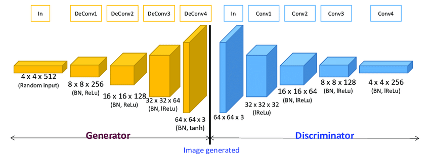
What are they? DCGANs use deep convolutional neural networks (CNNs) for both the generator and the discriminator.
How do they work? Convolutional layers are excellent at capturing spatial hierarchies in images. In DCGANs, the generator uses transposed convolutions to upsample random noise into images, while the discriminator uses standard convolutions to classify images as real or fake.
Benefits: This architecture improves the quality of generated images significantly. The generator can produce more detailed and realistic images, while the discriminator gets better at distinguishing real from fake images.
Loss Function: The loss functions in DCGANs are the same as in traditional GANs:
\[ \mathcal{L}_D = - \mathbb{E}_{x \sim p_{\text{data}}(x)}[\log D(x)] - \mathbb{E}_{z \sim p_z(z)}[\log(1 - D(G(z)))] \]
Term 1: \(- \mathbb{E}_{x \sim p_{\text{data}}(x)}[\log D(x)] \) is maximized when the discriminator correctly identifies real images as real. \(D(x)\) should be close to 1 for real images.
Term 2: \(- \mathbb{E}_{z \sim p_z(z)}[\log(1 - D(G(z)))] \) is minimized when the discriminator correctly identifies fake images as fake. \(D(G(z))\) should be close to 0 for fake images.
\[ \mathcal{L}_G = - \mathbb{E}_{z \sim p_z(z)}[\log D(G(z))] \]
This term is minimized when the generator successfully fools the discriminator into believing that fake images are real. \(D(G(z))\) should be close to 1 for fake images.

Wasserstein GANs (WGANs)

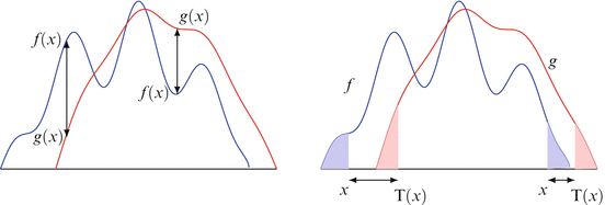
What are they? WGANs modify the loss function of GANs to use the Wasserstein distance (Earth Mover's distance) instead of the standard binary cross-entropy loss.
How do they work? The Wasserstein distance provides a smoother and more meaningful gradient, which helps stabilize the training process. WGANs also enforce a Lipschitz constraint by clipping the weights of the discriminator.
Benefits: WGANs address issues like mode collapse and provide more stable and reliable training, leading to higher quality generated images.
Loss Function: The WGAN loss function is based on the Wasserstein distance.
\[ \mathcal{L}_D = -\mathbb{E}_{x \sim p_{\text{data}}(x)}[D(x)] - \mathbb{E}_{z \sim p_z(z)}[D(G(z))] \]
Term 1: \( -\mathbb{E}_{x \sim p_{\text{data}}(x)}[D(x)] \) is minimized when the discriminator assigns a high score to real images.
Term 2: \( - \mathbb{E}_{z \sim p_z(z)}[D(G(z))] \) is minimized when the discriminator assigns a low score to fake images.
\[ \mathcal{L}_G = - \mathbb{E}_{z \sim p_z(z)}[D(G(z))] \]
This term is minimized when the generator produces fake images that the discriminator rates as high-quality (assigning them high scores).

Conditional GANs (CGANs)

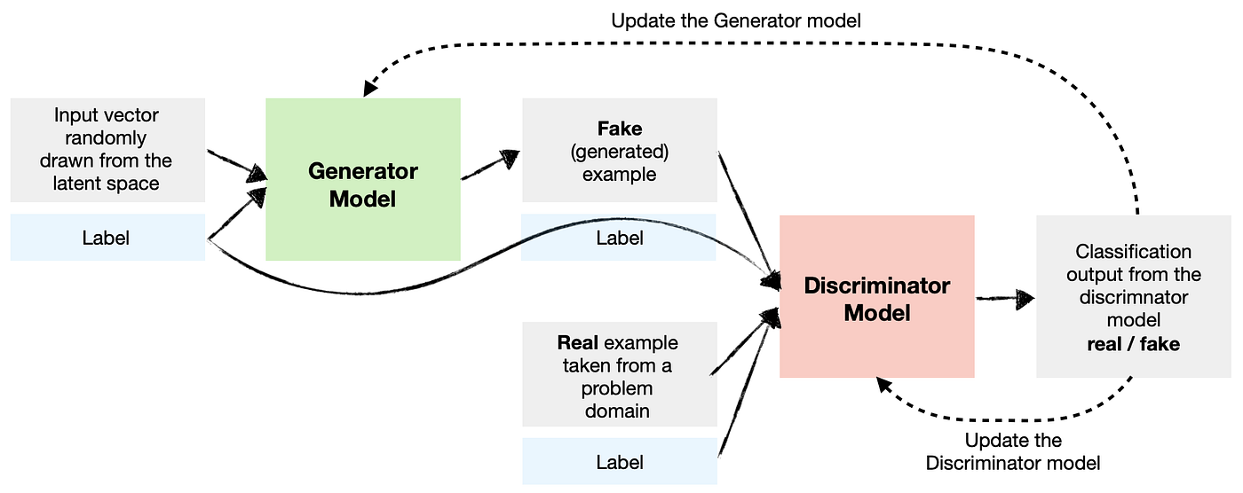
What are they? CGANs incorporate additional information (like class labels) into the generation process.
How do they work? Both the generator and the discriminator receive this extra information. For instance, if you want to generate images of cats, you provide the label "cat" to both networks. The generator then produces images of cats, and the discriminator learns to differentiate between real and fake cat images.
Benefits: This approach allows for more control over the generated images. You can direct the GAN to create specific types of images, making CGANs useful for tasks where you need targeted generation.
Loss Function: The loss functions for CGANs extend the traditional GAN losses to include the conditioning information ground truth label \(y\).
\[ \mathcal{L}_D = - \mathbb{E}_{x, y \sim p_{\text{data}}(x, y)}[\log D(x|y)] - \mathbb{E}_{z \sim p_z(z), y \sim p_{\text{data}}(y)}[\log(1 - D(G(z|y)))] \]
Term 1: \(- \mathbb{E}_{x, y \sim p_{\text{data}}(x, y)}[\log D(x|y)] \) is maximized when the discriminator correctly identifies real images conditioned on y as real. \( D(x|y) \) should be close to 1 for real images conditioned on \( y \).
Term 2: \(- \mathbb{E}_{z \sim p_z(z), y \sim p_{\text{data}}(y)}[\log(1 - D(G(z|y)))] \) is minimized when the discriminator correctly identifies fake images conditioned on y as fake. \( D(G(z|y)) \) should be close to 0 for fake images conditioned on \( y \).
\[ \mathcal{L}_G = - \mathbb{E}_{z \sim p_z(z), y \sim p_{\text{data}}(y)}[\log D(G(z|y))] \]
This term is minimized when the generator successfully fools the discriminator into believing that fake images conditioned on y are real. \( D(G(z|y)) \) should be close to 1 for fake images conditioned on \( y \).

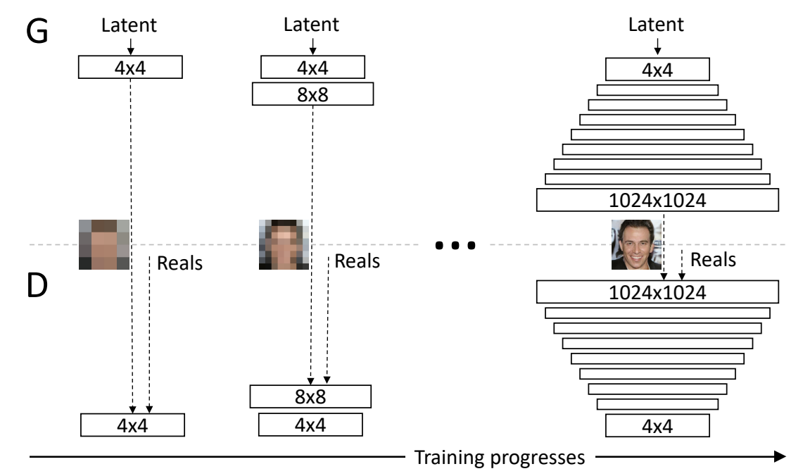
Progressive Growing of GANs (ProGANs)

What are they? ProGANs train GANs by gradually increasing the resolution of the generated images.
How do they work? Training starts with low-resolution images, and layers are progressively added to both the generator and the discriminator to increase the resolution step-by-step. This incremental approach helps in stabilizing the training process.
Benefits: ProGANs produce high-resolution images with finer details and help overcome training instability. The gradual growth allows the networks to learn more effectively at each resolution stage.
Loss Function: ProGANs use the same loss functions as traditional GANs, but the training is done progressively by adding layers:
\[ \mathcal{L}_D = - \mathbb{E}_{x \sim p_{\text{data}}(x)}[\log D(x)] - \mathbb{E}_{z \sim p_z(z)}[\log(1 - D(G(z)))] \]
Term 1: \( - \mathbb{E}_{x \sim p_{\text{data}}(x)}[\log D(x)] \) is maximized when the discriminator correctly identifies real images as real. \( D(x) \) should be close to 1 for real images.
Term 2: \( - \mathbb{E}_{z \sim p_z(z)}[\log(1 - D(G(z)))] \) is minimized when the discriminator correctly identifies fake images as fake. \( D(G(z)) \) should be close to 0 for fake images.
\[ \mathcal{L}_G = - \mathbb{E}_{z \sim p_z(z)}[\log D(G(z))] \]
This term is minimized when the generator successfully fools the discriminator into believing that fake images are real. \( D(G(z)) \) should be close to 1 for fake images.

Exciting Applications of GANs

Image Generation: They can create realistic images from scratch.
Image-to-Image Translation: Convert images from one type to another, like turning a sketch into a photo.
Super-Resolution: Enhance the resolution of images, making them sharper and more detailed.
Data Augmentation: Generate extra training data to help improve other machine learning models.

And that’s a wrap! GANs are an exciting and rapidly evolving field in AI, and their ability to generate realistic data opens up a world of possibilities. Whether you’re an AI enthusiast, a researcher, or just someone who loves cool tech, GANs have something to fascinate everyone. Happy GAN-ing! 🎨✨